1. Main characteristics of optical satellites¶

1.1. Remote sensing, Earth observation and GIS¶

Remote sensing and Earth observation are often used interchangeably, but they refer to different concepts:

Remote sensing is the

“The gathering of information without actual physical contact with what is being observed. This involves the use of radars, sonars, spectroscopy, and the use of airborne and satellite photography.”
(Credit: Oxford Dictionary of Earth Sciences. © Oxford University Press).

while Earth observation (EO) is the

“The gathering of information about planet Earth’s physical, chemical and biological systems via remote sensing technologies, usually involving satellites carrying imaging devices. Earth observation is used to monitor and assess the status of, and changes in, the natural and manmade environment.”
(Credit: European Commission).

That means Earth observation is the process of collecting information on our planet using contactless remote sensing technologies.

1.2. Satellites for Earth observation¶

Today, hundreds of satellites are orbiting or planet. They differ for:

Orbits and revisit time,
Imaging cameras,
Spatial resolution and swath width,
Spectral characteristics,

All these characteristics are defined during the mission design, depending on the satellite mission’s specific applications.

For example, to monitor the weather at a global scale and in real-time, we need satellites with a very high orbit, a low spatial resolution with a large swath, and a few spectral bands (Fig. 1.2.1).

Hint

Click here to see real-time meteo imageries over Europe (Credit: EUMETSAT – CC BY-SA IGO 3.0).

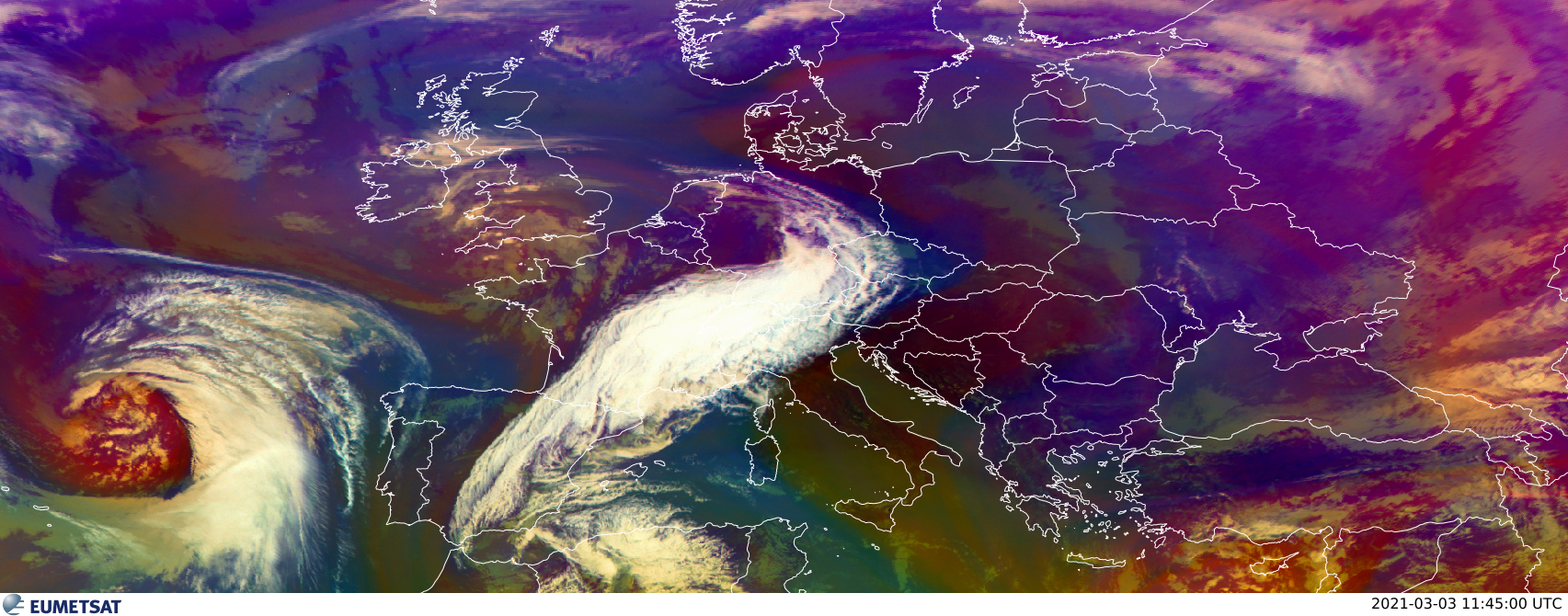
Fig. 1.2.1 Earth observation missions developed by the European Space Agency (credit: EUMETSAT [2021] – CC BY-SA IGO 3.0).¶

On the opposite, to monitor our urban areas, we need satellites with a low orbit, a high spatial resolution with a small swath, and many spectral bands (Fig. 1.2.2).

Hint

Click here to see a 30 cm satellite image over Madrid (Spain) (Credit: © European Space Imaging).

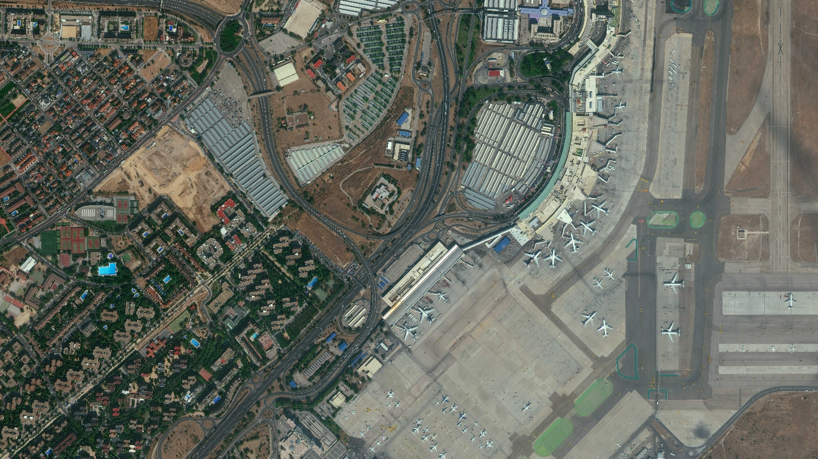
Fig. 1.2.2 Earth observation missions developed by the European Space Agency (credit: © European Space Imaging).¶

1.2.1. Satellite orbits and revisit time¶

a. High Earth orbit (HEO)
Satellites in high Earth orbit circle Earth at an altitude > 35,800 km.

EXAMPLE: In this orbit we find satellites for space exploration.

a. Geosynchronous orbit (IGSO)
Satellites in geosynchronous orbit circle Earth at an altitude of 35,800 km and a speed of about 3 km/s. This makes geostationary satellites rotate synchronized with the rotation of the Earth.

EXAMPLE: Many satellites used for telecommunications/broadcasting have a geosynchronous orbit.

b. Geostationary orbit (GEO)
This is a particular kind of geosynchronous orbit, where satellites are parked over the equator. This makes geostationary satellites to be ‘stationary’ over a fixed location on Earth.

EXAMPLE: Most of the satellites used for weather forecasts have a geostationary orbit.

c. Medium Earth orbit (MEO)
Satellites in a medium Earth orbit circle the Earth at an altitude between 1,000 km and 35,800 km, with variable speed.

EXAMPLE: Navigation satellites, like the European Galileo system or the American NAVSTAR-GPS, have a medium Earth orbit.

d. Low Earth orbit (LEO)
Satellites in a low Earth orbit circle close to Earth’s surface, at an altitude between 200 km and 1,000 km and a speed of about 7.8 km/s.
At this speed, a satellite takes approximately 90 minutes to circle Earth. Thus, travels around Earth about 16 times a day.

EXAMPLE: satellites for Earth observation usually have a low Earth orbit.

e. Sun-synchronous orbit (SSO)
This is a particular kind of low Earth orbit, where satellites circle from north to south and are always in the same ‘fixed’ position relative to the Sun. This means that the satellites still visits the same geographic location at the same local time.

Most of satellites for Earth observation have a Sun-synchronous (SSO) low Earth orbit (LEO), with an altitude between 600 km and 800 km , a speed of approximately 7.5 km/s and about 16 orbits per day.

Note

Depending on the time needed for imaging the same geographic location (called revisiting time), satellites are classified as:

High revisit time: < 3 days
Medium revisit time: 4 - 16 days
Low revisit time: > 16 days

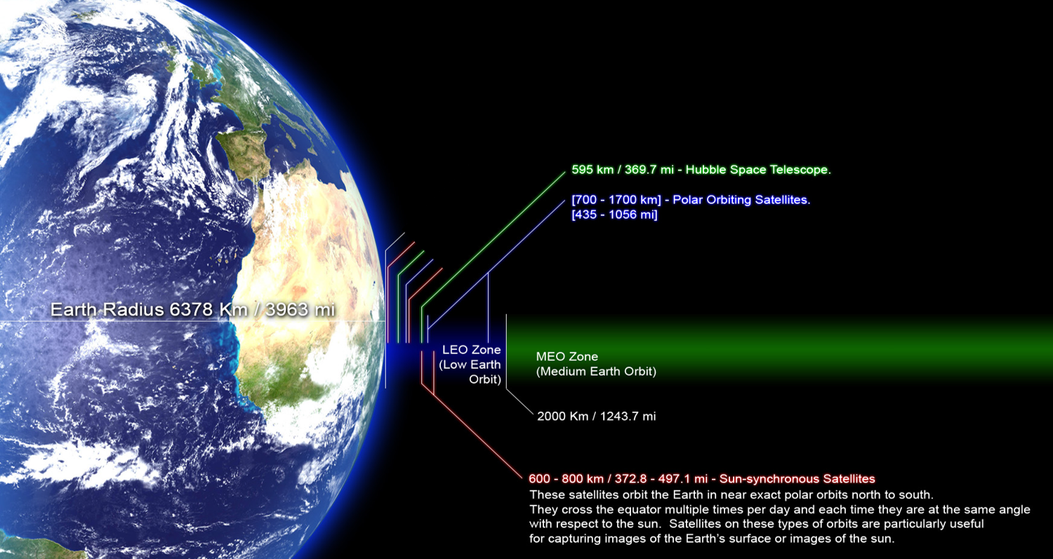
Fig. 1.2.1.1 Satellite orbits (credit: adapted from Mark Mercer, 2011 - CC BY-SA 4.0).¶

(Credit: NASA, illustration by Robert Simmon).

Hint

Small activity
See the real-time location of about 19,300 manmade objects orbiting the Earth with ESRI Satellite Map (updated on 14 July 2020).

Hint

Small activity
Search for a specific satellite with the live real time satellite tracking and predictions (up to date).

Hint

Small activity
Plan your open data satellite acquisitions with Spectator Earth (up to date).

1.2.2. Digital images and the EM spectrum¶

A greyscale digital image is a matrix (i.e. table) of individual elements (called pixels) representing the brightness of a specific geographic location recorded in a particular range of wavelengths of the electromagnetic spectrum (called spectral band, or just band) (Fig. 1.2.2.1).

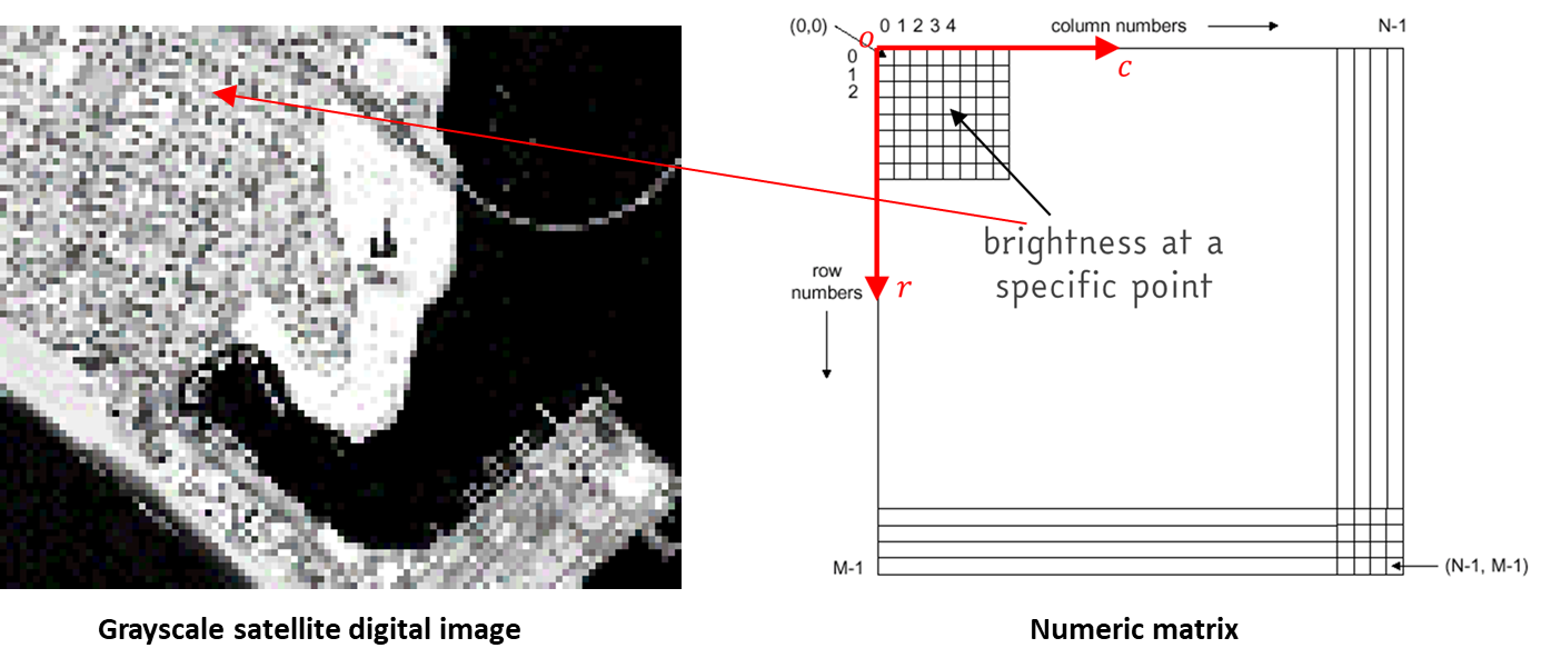
Fig. 1.2.2.1 The digital image as a table of numbers.¶

But what are the electromagnetic spectrum and wavelengths?

Consider the electromagnetic spectrum as the full range of “light” that exists in the universe (Fig. 1.2.2.2): from Gamma rays (shorter wavelengths) to Radio waves (longer wavelengths).
We can think of the different wavelengths as different “colours”.

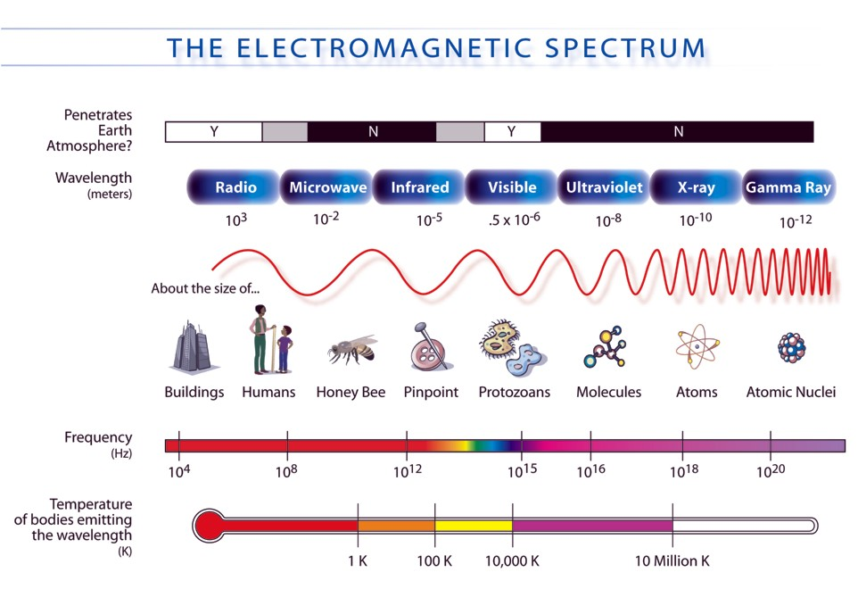
Fig. 1.2.2.2 The electromagnetic spectrum (credit: NASA – CC BY-SA 3.0).¶

Hint

Small activity
See how the electromagnetic waves combines with the EMANIM tool .

Unfortunately, most of these “colours” and “light” are invisible to our eyes!
We humans can see only the colours of the VISIBLE light. However, many other “colours” exists, and some animals can see them. For instance, snakes can sense the INFRARED (i.e. the heat) and some insects can see the ULTRAVIOLET.

Fig. 1.2.2.3 and Fig. 1.2.2.4 show how human eyes and animal eyes sense different wavelengths of the electromagnetic spectrum.

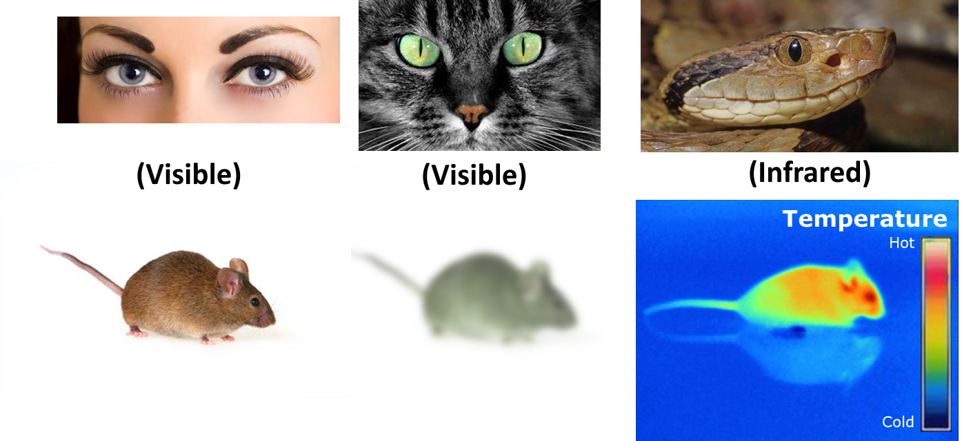
Fig. 1.2.2.3 The electromagnetic spectrum sensed by humans, cats and snakes.¶

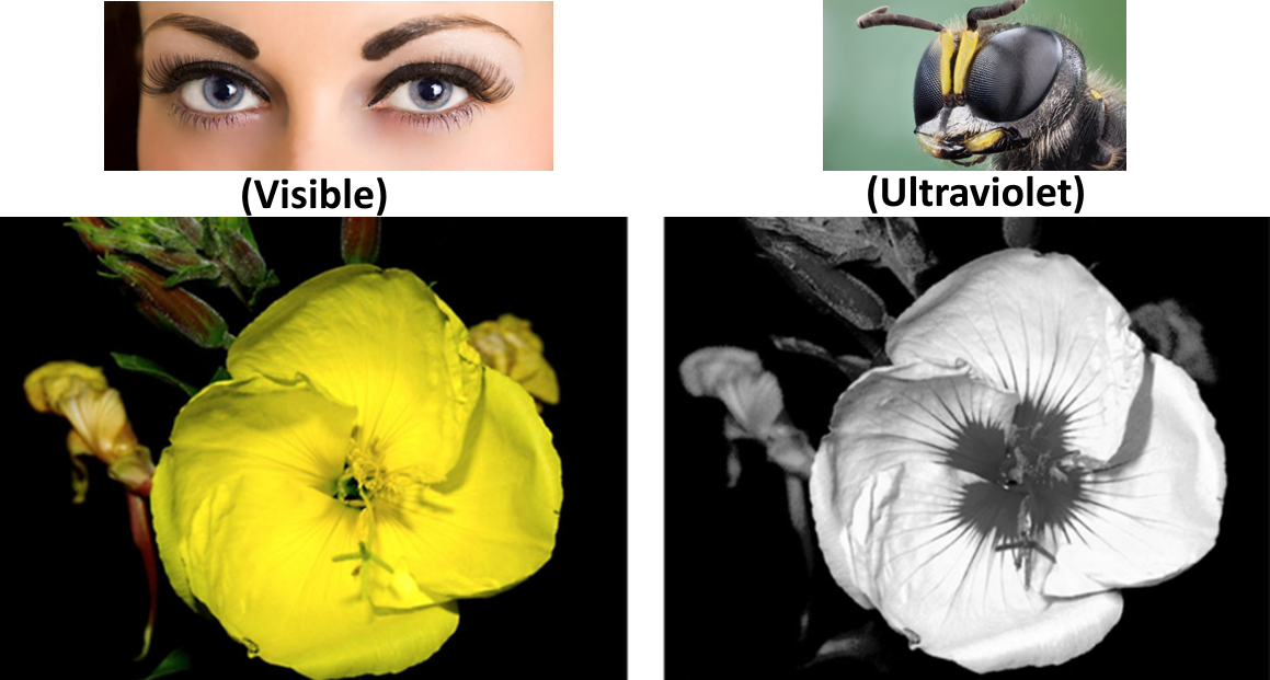
Fig. 1.2.2.4 The electromagnetic spectrum sensed humans and bees.¶

Hint

Small activity
See planet Earth live from the International Space Station with the External High Definition Camera (real time streaming).

1.2.3. Spectral characteristics¶

Optical satellites use special “cameras”, called multispectral cameras.

Multispectral cameras produce multispectral (=multiband) grayscale images. That is to say, a multitude of greyscale images - collected at the same time - recording the reflected sunlight in a specific range of wavelengths (i.e. the spectral bands) (Fig. 1.2.3.1).

In other words, a multiband image describes the intensity of the different “colours” sensed in the different “lights” of the electromagnetic spectrum.

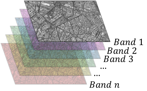
Fig. 1.2.3.1 Example of multiband image.¶

Hint

Small activity
Try the Remote Sensing Virtual Lab to see how the land looks like in different wavelengths (cretits: Karen Joyce).

In photography, spectral bands are usually called colour channels.
A smartphone takes pictures in only 3 VISIBLE colour channels:

Red channel (R),
Green channel (G),
Blue channel (B).

But satellites allow extending our visual perception to many more “colours”, even to wavelengths where our eyes are blind!

Hint

Small activity
To see the colour channels, try RGB channels splitter with a photo taken with your smartphone (Fig. 1.2.3.2)! Try using both outputs “as greyscale”, and “with their own colour”.
You might also use this test picture.

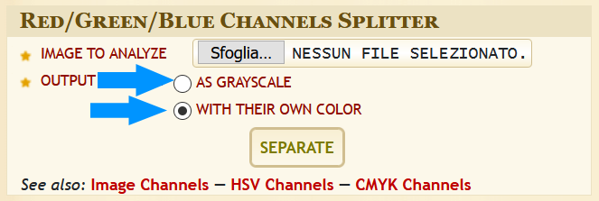
Fig. 1.2.3.2 Colour channels splitter.¶

Hint

Small activity
Try Combine RGB channels to combine greyscale satellite images into a satellite colour image:

Download Sentinel-2 image of Venice (Blue spectral band),
Download Sentinel-2 image of Venice (Green spectral band),
Download Sentinel-2 image of Venice (Red spectral band).

What happens to colours if you mix up the spectral spectral bands?

1.2.4. Spatial resolution and area coverage¶

The spatial resolution specifies the pixel size of satellite images at the Earth surface. It describes the ability to separate small spatial details.
Depending on their pixel size, remote sensing cameras are classified as:

Very high spatial resolution: < 1 m,
High spatial resolution: 1 -5 m,
Medium spatial resolution: 5 - 100 m,
Low spatial resolution: > 100 m.

Fig. 1.2.4.1 The London Eye (UK). The effect of spatial resolution on image detail.¶

The area imaged on the ground is called swath. Thus, the swath defines the geographic extent of a single satellite image.
Generally speaking:

Very high & high resolution imaging cameras have a narrow swath: about dozen of km,
Medium resolution imaging cameras have a large swath: few hundreds of km,
Low resolution imaging cameras have a wide swath: up to thousands of km.

Fig. 1.2.4.2 The London Eye (UK). The effect of spatial resolution on swath.¶

Very high & high resolution cameras are typically needed for applications requiring great spatial detail of a particular site, such as mapping buildings damaged by an earthquake. Such cameras would generally be onboard of low Earth orbit satellites and have a narrow swath. In such an orbit, nadir images can be acquired with a low revisit time (when the satellite overpasses the area of interest).

On the opposite, geostationary satellites have low resolution cameras with wide swath. In such an orbit, images over the area of interest are acquired with a very high revisit time (near real-time). These satellites are suitable for continental and global studies.

Medium resolution cameras with pixel size between 10 m and 30 m usually have a swath of about 200-300 km. They are often a good compromise for many application needs.

Tip

Spatial resolution vs orbital altitude
The spatial resolution is proportional to the orbital altitude. Thus, geostationary satellites have a low spatial resolution, while low Earth orbit satellites could achieve very high spatial resolution.

1.3. Copernicus and the Sentinels¶

1.3.1. The Copernicus programme¶

Copernicus is the flagship European Union’s Earth Observation Programme, looking at our planet and its environment. Every day, Copernicus collects a large amount of global data from ground stations, satellites, airborne and seaborne systems. Then, transforms these data into information to support public authorities, international organisations and the industry in improving the quality of life for all European citizens.

Copernicus’s information can be used by end-users for a wide range of applications and various subject areas, including:

Urban area management,
Sustainable development and nature protection,
Regional and local planning,
Agriculture,
Forestry,
Fisheries,
Health,
Civil protection,
Infrastructure,
Transport and mobility,
Tourism.

1.3.2. Multispectral Sentinel satellites¶

Sentinel-2
The Sentinel-2 satellites (twin satellites Sentinel-2A and Sentinel-2B) provide multispectral medium resolution imagery for land services. Table 1.3.2.1 shows its main specifications.
Their orbit is Sun-synchronous, and the constellation (2 identical satellites) has an overall revisit time of 5 days at the equator and about 2-3 days at mid-latitudes.

The mission objectives for Sentinel-2 are systematic:

Land observation of vegetation and soil and water cover, inland waterways and coastal areas,
Land use and change detection maps,
Providing support in generating land cover,
Disaster relief support,
Climate change monitoring.

Table 1.3.2.1 Sentinel-2 spectral bands.¶
Band	Spectral region	Colour	Spatial resolution	Swath width	Application
1	432 - 453 nm	Visible (Violet)	60 m	290 km	Estimation of atmospheric aerosol
2	459 - 525 nm	Visible (Blue)	10 m	290 km	Mapping reflected Blue light
3	542 - 578 nm	Visible (Green)	10 m	290 km	Mapping reflected Green light
4	649 - 680 nm	Visible (Red)	10 m	290 km	Mapping reflected Red light
5	697 - 712 nm	Near infrared 1 (red edge)	20 m	290 km	Classification of vegetation
6	733 - 748 nm	Near infrared 2 (red edge)	20 m	290 km	Classification of vegetation
7	773 - 793 nm	Near infrared 3 (red edge)	20 m	290 km	Classification of vegetation
8	780 - 886 nm	Near infrared 4	10 m	290 km	Sensitive to chlorophyll and biomass
8A	854 - 875 nm	Near infrared 5 (red edge)	20 m	290 km	Classification of vegetation
9	935 - 955 nm	Near infrared 6	60 m	290 km	Estimation of atmospheric water vapor
10	1,358 - 1,389 nm	Short-wave infrared 1	60 m	290 km	Detection of clouds (cirrus)
11	1,568 - 1,659 nm	Short-wave infrared 2	20 m	290 km	Sensitive to lignin, discrimination of snow / ice / clouds
12	2.115 - 2.290 nm	Short-wave infrared 3	20 m	290 km	Distinction of live and dead biomass, discrimination of snow / ice / clouds

Hint

See how Sentinel-2 collects multispectral images

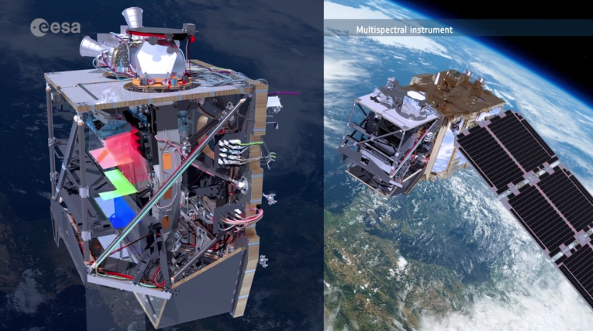
Fig. 1.3.2.1 Sentinel-2 multispectral imager (MSI) (credit: ESA/ATAG medialab – CC BY-SA IGO 3.0)¶

Sentinel-3
The Sentinel-3 satellites (twin satellites Sentinel-3A and Sentinel-3B) provide multispectral low resolution imagery for ocean and land services.
Their orbit is Sun-synchronous, and the constellation (2 identical satellites) has an overall revisit time less than 2 days.

The mission objectives for Sentinel-3 are global coverage of:

Ocean and land-surface temperature,
Ocean and land-surface colour,
Sea-water quality and pollution monitoring,
Inland water monitoring, including rivers and lakes,
Aid ocean forecasts with acquired data,
Climate monitoring and modelling,
Land-use change monitoring,
Forest cover mapping,
Fire detection,
Weather forecasting,
Measuring Earth’s thermal radiation for atmospheric applications.

The Ocean and Land Colour Instrument (OLCI) has a 300-meters spatial resolution in 21 spectral bands, with a swath width of 1,270 km. Table 1.3.2.2 shows its main specifications.

Table 1.3.2.2 Sentinel-3 OLCI spectral bands.¶
Band	Spectral region	Colour	Spatial resolution	Swath width	Application
1	393 - 408 nm	Visible 1 (Violet)	300 m	1,270 km	Aerosol correction, improved water constituent retrieval
2	408 - 418 nm	Visible 2 (Violet)	300 m	1,270 km	Yellow substance and detrital pigments (turbidity)
3	438 - 448 nm	Visible 3 (Violet-Blue)	300 m	1,270 km	Chlorophyll absorption maximum, biogeochemistry, vegetation
4	485 - 495 nm	Visible 4 (Cyan)	300 m	1,270 km	High Chlorophyll
5	505 - 515 nm	Visible 5 (Green)	300 m	1,270 km	Chlorophyll, sediment, turbidity, red tide
6	555 - 565 nm	Visible 6 (Green)	300 m	1,270 km	Chlorophyll reference (Chlorophyll minimum)
7	615 - 625 nm	Visible 7 (Red)	300 m	1,270 km	Sediment loading
8	615 - 625 nm	Visible 8 (Red)	300 m	1,270 km	Chlorophyll, sediment, yellow substance/vegetation
9	670 - 678 nm	Visible 9 (Red)	300 m	1,270 km	Improved fluorescence retrieval
10	678 - 685 nm	Visible 10 (Red)	300 m	1,270 km	Chlorophyll fluorescence peak
11	704 - 714 nm	Near infrared 1 (red edge)	300 m	1,270 km	Chlorophyll fluorescence baseline
12	750 - 758 nm	Near infrared 2 (red edge)	300 m	1,270 km	Oxigen absorption, clouds, vegetation
13	760 - 763 nm	Near infrared 3 (red edge)	300 m	1,270 km	Aerosol correction
14	763 - 766 nm	Near infrared 4 (red edge)	300 m	1,270 km	Atmospheric correction
15	766 - 769 nm	Near infrared 5 (red edge)	300 m	1,270 km	Fluorescence over land
16	771 - 786 nm	Near infrared 6 (red edge)	300 m	1,270 km	Atmospheric/aerosol correction
17	855 - 875 nm	Near infrared 7	300 m	1,270 km	Atmospheric/aerosol correction, clouds
18	880 - 890 nm	Near infrared 8	300 m	1,270 km	Water vapour absorption, vegetation monitoring
19	895 - 905 nm	Near infrared 9	300 m	1,270 km	Water vapour absorption, vegetation monitoring
20	930 - 950 nm	Near infrared 10	300 m	1,270 km	Water vapour absorption, atmospheric correction
21	1,000 - 1,040 nm	Near infrared 11	300 m	1,270 km	Atmospheric/aerosol correction

The Sea and Land Surface Temperature Radiometer (SLSTR) instrument record the surface temperature with 1 km spatial resolution. Table 1.3.2.3 shows its main specifications.

Table 1.3.2.3 Sentinel-3 SLSTR spectral bands.¶
Band	Spectral region	Colour	Spatial resolution	Swath width	Application
S1	545 - 564 mn	Visible 1 (Green)	500 m	1,270 km	Cloud screening, vegetation monitoring, aerosol
S2	650 - 669 nm	Visible 2 (Red)	500 m	1,270 km	Vegetation monitoring, aerosol
S3	858 - 878 nm	Near infrared	500 m	1,270 km	Cloud
S4	1,364 - 1,385 nm	Short-wave infrared 1	500 m	1,270 km	Cirrus detection over land
S5	1,583 - 1,644 nm	Short-wave infrared 2	500 m	1,270 km	Cloud, ice, snow, vegetation monitoring
S6	2,231 - 2,281 nm	Short-wave infrared 3	500 m	1,270 km	Vegetation state and clouds
S7	3,543 - 3,941 nm	Thermal infrared 1	1 km	1,270 km	Active fires
S8	10,466 - 11,242 nm	Thermal infrared 2	1 km	1,270 km	Surface temperature, active fires
S9	11,570 - 12,475 nm	Thermal infrared 3	1 km	1,270 km	Surface temperature
F1	3,543 - 3,941 nm	Thermal infrared 4	1 km	1,270 km	Active fires
F2	10,466 - 11,242 nm	Thermal infrared 5	1 km	1,270 km	Surface temperature, active fires

Hint

Look inside Sentinel-3

(Credit: ESA/ATG medialab – CC BY-SA IGO 3.0).

Sentinel-5P
Sentinel-5P is the precursor mission of Sentinel-5 and provides multispectral extremely low resolution imagery for atmospheric and climate services. Table 1.3.2.4 shows its main specifications.

The mission objective for Sentinel-5P is to provide daily global information on air pollutants for the atmosphere monitoring and climate change services:

Aerosols,
Clouds,
Ozone \((O_3)\),
Nitrogen dioxide \(({\rm NO}_2)\),
Carbon monoxide \((CO)\),
Sulfur dioxide \(({\rm SO}_2)\),
Methane \(({\rm CH}_4)\),
Formaldehyde \(({\rm CH}_2O)\).

Table 1.3.2.4 Sentinel-5P spectral bands.¶
Band	Spectral region	Colour	Spatial resolution	Swath width
1	270 - 300 nm	Ultraviolet 1	28 km x 7 km	2,670 km
2	300 - 370 nm	Ultraviolet 2	3.5 km x 7 km	2,670 km
3	370 - 500 nm	Ultraviolet & Visible (Violet-Blue)	3.5 km x 7 km	2,670 km
4	685 - 710 nm	Near Infrared 1	3.5 km x 7 km	2,670 km
5	745 - 773 nm	Near Infrared 2	3.5 km x 7 km	2,670 km
6	1,590 - 1,675 nm	Short-wave infrared 1	7 km x 7 km	2,670 km
7	2,305 - 2,385 nm	Short-wave infrared 2	7 km x 7 km	2,670 km

Hint

Small activity
See the benefits of the lockdown in China on air quality

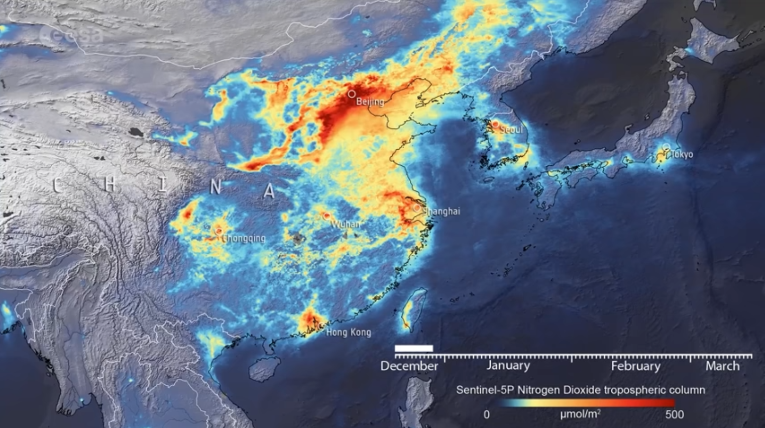
Fig. 1.3.2.2 See the benefits of the lockdown in China on air quality (credit: ESA/ATAG medialab – CC BY-SA IGO 3.0).¶